现代 Diffusion 推理最小背景
阅读前提:你已了解 flow matching / score matching 的基本概念(知道什么是 vector field、什么是 score function、为什么扩散过程可以看作 ODE/SDE)。本文只聚焦推理阶段,不讨论训练。
目录
0. 推理全景:1 条 prompt 怎么变成 1 张图(或一段视频)
在开始拆零件之前,先把整条流水线扫一遍:
下面逐个拆开来看。
1. prompt → tokenizer → text encoder → prompt embeddings
这是整条流水线的文本入口,也是唯一一次和 LLM 世界有交集的地方,但这里的 text encoder 只是 conditioning,不是生成主体。
1.1 Tokenizer
将自然语言 prompt 拆成 token id 序列。现代 diffusion 模型通常使用 subword tokenizer(BPE 或 SentencePiece),和 LLM 的 tokenizer 没有本质区别。
prompt = "a cat sitting on a table"
token ids = [320, 4567, 1234, ...]   # shape: (1, L)
L 通常是模型定义的最大 prompt 长度,不足则 padding + attention mask,超出则截断。
1.2 Text Encoder
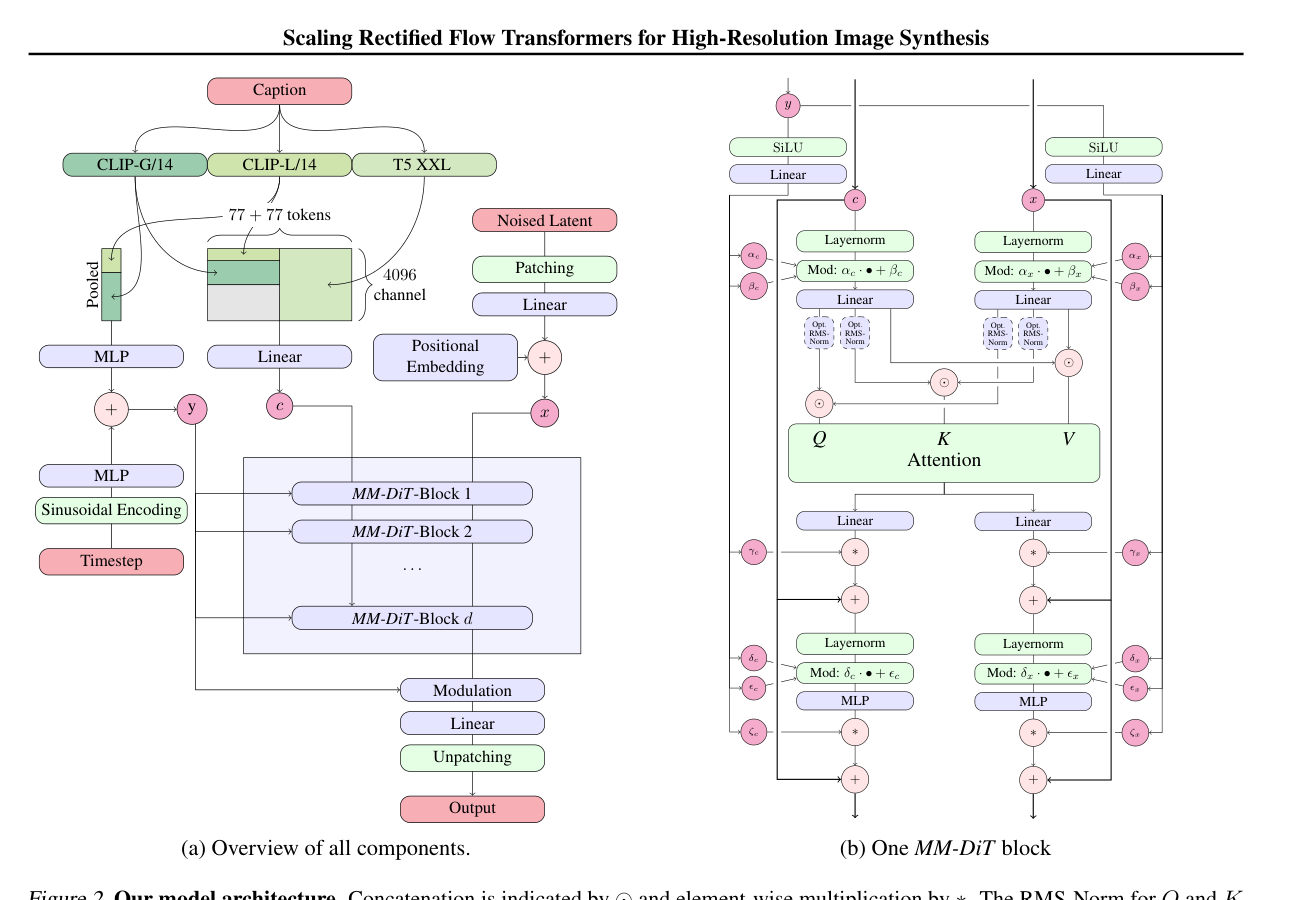
将 token ids 映射为连续向量,产出 prompt embeddings。现代文生图/视频模型使用的 text encoder 组合:
| 模型族 | Text Encoder | 输出维度 | 说明 |
|---|---|---|---|
| SD3 / FLUX | CLIP-L + CLIP-G + T5-XXL | CLIP: 768/1280, T5: 4096 | T5 很重,FLUX schnell 或 SD3-Medium 可省略 T5 |
| Sana | Gemma-2B (LLM) | 2304 | 直接用 1 个小 LLM 做 text encoder |
| CogVideoX | T5-XXL | 4096 | 视频模型用 T5 |
| LTX-Video | T5-XXL | 4096 | 同上 |
Text encoder 的调用次数:text encoder 只在推理开始时 run 1 次,它的输出(prompt embeddings)会在整个去噪循环中被复用。CFG 还可能需要 2 组编码:1 组来自 prompt(positive/conditional),另一组来自空字符串(negative/unconditional)。这 2 组 embedding 都可以 cache。
1.3 输出 shape
prompt_embeds:     (B, L, D_text)     # 例如 (1, 77, 4096)
pooled_prompt_embeds: (B, D_pool)     # 有些模型额外输出 pooled embedding
B = batch size,通常为 1(单张生成)。
2. noise / latent 初始化
2.1 Latent space 概念
现代 diffusion 通常在 latent space(VAE 压缩后的空间)而不是像素空间操作。Latent diffusion 用 VAE 把高分辨率图像或视频压成低分辨率 latent,在 latent 上完成 diffusion,再由 VAE decoder 还原。
为什么要用 latent space?
- 计算效率:latent 尺寸通常是像素的 1/8(每边)。512×512 像素 → 64×64 latent,token 数从 262k 降到 4k。
- 显存占用:latent 通道数通常为 4 或 16,虽然高于 RGB 的 3 个通道,但 VAE 会压缩 H、W,因此总 token 数更少。自注意力复杂度与 token 数的平方成正比,空间压缩会直接缩小 attention 矩阵。
- 解耦:VAE 可以独立训练、独立替换、独立升级。VAE encoder/decoder 和 diffusion 模型是完全解耦的 2 个模块。
2.2 Image latent 初始化
典型配置(以 SD3/FLUX 为例):
latent_shape: (B, C, H, W) = (1, 4, 64, 64)- C = 4:VAE latent 通道。某些模型用 C=16(如 FLUX 的高 latent 通道变体)。
- H = W = 64:512×512 像素经 8× VAE 下采样。如果图像是 1024×1024,则 latent 为 (1, 4, 128, 128)。
- 下采样比例:VAE 的压缩因子通常是 8(沿每边),也有用 16 的。
2.3 Video latent 初始化
latent_shape: (B, C, T, H, W) = (1, 4, 16, 32, 32)- C = 4:同图像 latent。
- T = 16:16 帧视频。这是常见的小规格设置。
- H = W = 32:256×256 像素经 8× VAE 压缩。实际生产模型可能用更多帧和更高分辨率。
- 注意:不同模型对维度的约定不同,有些用
(B, C, T, H, W),有些用(B, T, C, H, W)。在你的diffusion_engine/里需要统一约定或做显式 rearrange。
spacetime patch:视频 DiT 通常在进入 transformer 之前,把 (B, C, T, H, W) 的 latent 进一步按 spacetime patch 切块。例如取 patch size = (1, 2, 2),表示时间维度不切(patch_t=1),空间维度 2×2 1 组。这样:
(B, C, T, H, W) → (B, N_patches, D_patch)其中 \(N_{\mathrm{patches}} = (T / \mathrm{patch}_t) \times (H / \mathrm{patch}_h) \times (W / \mathrm{patch}_w)\),每个 patch 被展平并投影到 transformer 的 hidden dimension。这和 ViT 的 image patchify 思路一致,只是多了一维时间轴。
2.4 随机性来源与 seed
初始化 latent 使用标准高斯噪声:
import torch
z_T = torch.randn(1, 4, 64, 64,
    generator=torch.Generator().manual_seed(seed))
Seed 决定初始噪声。在相同运行条件下,同样的 seed、prompt 和参数应得到相同输出。diffusion_engine/ 的 pipeline 因此需要暴露 seed 参数。
3. timestep / sigma schedule
3.1 基本概念
在 flow matching / rectified flow 框架中,时间 \(t \in [0, 1]\) 表示从噪声(\(t=0\))到数据(\(t=1\))的进度。推理时我们倒退:从 \(t=1\)(纯噪声)逐步走到 \(t=0\)(干净 latent)。
每一步对应当前的时间值 \(t_i\),以及对应的噪声水平 \(\sigma\)(sigma)。不同的 scheduler 把时间轴离散化成不同的步数。
3.2 Image 模型的常用 schedule
| 模型 | Scheduler | 典型步数 | 说明 |
|---|---|---|---|
| SD3 | FlowMatchEulerDiscreteScheduler | 28~50 | rectified flow Euler |
| FLUX schnell | FlowMatchEulerDiscreteScheduler | 4~8 | 蒸馏后的少步 scheduler |
| Sana | FlowMatchEulerDiscreteScheduler | 14~20 | 高效少步 |
image 默认:通常 20~50 步即可。蒸馏模型(如 FLUX schnell、LCM)可以降到 4~8 步。
3.3 Video 模型的常用 schedule
视频模型因为帧间一致性要求,通常需要更多步;蒸馏模型可以用更少步骤逼近原采样轨迹。
| 模型 | Scheduler | 典型步数 |
|---|---|---|
| CogVideoX | DDIM / FlowMatch | 50 |
| Wan | FlowMatchEuler | 50 |
| LTX-Video | FlowMatch (distilled) | 4~8 |
3.4 sigma 的作用
在每个推理步中,sigma(或 timestep)被作为 conditioning 输入 denoiser。具体方式通常是 timestep embedding:把 1 个标量 t 映射为高维向量,然后通过 adaLN(adaptive layer norm)或直接在 attention/MLP 中注入。
timestep → sinusoidal embedding → MLP → (scale, shift, gate)
                                             │
                                             ▼
                                    [DiT block] adaLN
4. denoiser / vector field / DiT forward
4.1 推理时 forward 做什么
给定当前 latent \(z_t\)、timestep \(t\)、prompt embeddings \(c\),denoiser 输出:
- Flow matching:vector field \(v_\theta(z_t, t, c)\),表示从当前位置指向数据方向的速度场。
- Score-based / DDPM-style:noise prediction \(\epsilon_\theta(z_t, t, c)\),预测当前 latent 中混入的噪声成分。
在 rectified flow 设定下,两者等价关系为 \(v_\theta = \hat{z}_1 - \hat{z}_0\)(终态减初态估计),或可以互相转换。本文档默认使用 flow matching / rectified flow 的 vector field 视角。
4.2 DiT(Diffusion Transformer)架构要点
现代 denoiser 常用 DiT 或 MMDiT(Multimodal DiT)替代老式 U-Net,包含以下模块:
每个 DiT block 通常包含:
- Self-Attention:latent tokens 之间的全局交互。
- Cross-Attention(可选):latent tokens attend to prompt tokens。有些设计用的是 MMDiT 的 joint attention,即 text 和 image tokens 放在同一个 sequence 中做 self-attention。
- MLP / FFN:逐 token 的非线性变换。
- adaLN:timestep embedding 通过 adaptive layer norm 注入每个 block。
4.3 为什么从 U-Net 转向 DiT / MMDiT
- Scaling 特性:Transformer 的 scaling law 已被大量验证。DiT 可以像 LLM 一样通过堆更多层、加宽 hidden dim 来提升质量,U-Net 的架构没有这么干净的 scaling 行为。
- 文本对齐:cross-attention 或 joint attention 让 DiT 能自然地融合文本信息和图像信息。U-Net 虽然也有 cross-attention,但整体设计受限于卷积 backbone。
- 全局 attention:Transformer 的 self-attention 天然全局,不需要像 U-Net 那样靠下采样来扩大感受野。这在处理长距离依赖(如一整张图或一整段视频)时优势明显。
- 多模态统一:MMDiT 把 text tokens 和 image tokens 放进同一个 transformer,这和现代多模态 LLM 的设计是同构的,更容易在预训练和微调中迁移。
4.4 推理时的 forward 调用
# 单步 forward
v_pred = denoiser(
    latent=z_t,                        # (B, C, H, W) 或 (B, C, T, H, W)
    timestep=t,                        # 标量或 (B,) tensor
    encoder_hidden_states=prompt_embeds, # (B, L, D_text)
)
# v_pred shape 与 z_t 相同
注意:在 CFG 场景下,你需要调 2 次 forward(见下节)。
5. classifier-free guidance (CFG)
5.1 问题
模型在推理时可能偏离 prompt,产生与文本描述不一致的内容。CFG 通过在 conditional 和 unconditional 预测之间插值来加强文本引导。
5.2 公式
CFG 作用于 noise prediction / vector field,而不是 latent。
\[ v_{\mathrm{cfg}} = v_{\mathrm{uncond}} + s\left(v_{\mathrm{cond}} - v_{\mathrm{uncond}}\right) \]其中:
v_cond:用真实 prompt 编码得到的 vector field。v_uncond:用空 prompt("")编码得到的 vector field。s:guidance scale(CFG scale),通常取值 1.0 ~ 7.5。
等价写法(noise prediction 视角):
\[ \epsilon_{\mathrm{cfg}} = \epsilon_{\mathrm{uncond}} + s\left(\epsilon_{\mathrm{cond}} - \epsilon_{\mathrm{uncond}}\right) \]5.3 为什么在 vector field 层面做
latent 是 denoiser 的输入和输出,而 CFG 修正的是 denoiser 的输出。如果在 latent update 后应用 CFG,插值对象已经包含 scheduler 更新,不再等价于对模型预测做引导。计算顺序如下:
v_cond   = denoiser(z_t, t, text_embeds)
v_uncond = denoiser(z_t, t, null_embeds)    # 两次 forward
v_cfg    = v_uncond + s × (v_cond − v_uncond) # CFG 合并
z_{t-1}  = scheduler.step(v_cfg, z_t, t)     # 再用合并结果更新 latent
5.4 边界情况
- \(s = 1.0\):\(v_{\mathrm{cfg}} = v_{\mathrm{cond}}\)。等价于只用 conditional 预测,不做 CFG。这在 distilled 模型(如 FLUX schnell)中是默认行为。
- \(s = 0.0\):\(v_{\mathrm{cfg}} = v_{\mathrm{uncond}}\)。等价于完全忽略 prompt,输出内容与 prompt 无关。仅用于测试或特殊需求。
- \(s > 1.0\):增强 prompt 引导力。值越大图像越"靠拢" prompt 描述,但可能过饱和、失真。7.5 是 SD 时代的常见值,现代 rectified flow 模型通常用 3.0~5.0。
5.5 显存代价
CFG 需要2 次 denoiser forward(conditional + unconditional),这意味着峰值显存约为基础 forward 的 2×(取决于你的 memory manager 如何复用 latent buffer)。这是 diffusion 推理最大的显存项之一。优化方向包括:
- Batched CFG:把 cond 和 uncond 拼成 batch=2 1 次 forward,利用 GPU 并行。
- Cache unconditional embedding:空 prompt 的 text embedding 在整个推理中不变,可以预计算并复用。
6. scheduler update
6.1 角色
Scheduler 负责根据 denoiser 的输出(vector field 或 noise prediction),把当前 latent \(z_t\) 更新到下一步 \(z_{t-1}\)(或等价地,更新到更接近数据的 \(z_{t - \Delta t}\))。
6.2 3 种常见 scheduler
| Scheduler | 更新方式 | 适用框架 | 特点 |
|---|---|---|---|
| Euler (flow) | \(z_{t-1} = z_t + \Delta t\,v_\theta(z_t, t, c)\) | Rectified Flow / Flow Matching | 最简单,一阶,少量步即可 |
| DDIM | \(z_{t-1} = \sqrt{\bar{\alpha}_{t-1}}\left(z_t - \sqrt{1-\bar{\alpha}_t}\,\epsilon\right) / \sqrt{\bar{\alpha}_t} + \sqrt{1-\bar{\alpha}_{t-1}}\,\epsilon\) | DDPM / Score-based | 确定性,比 DDPM 快,需要更多步 |
| Rectified Flow Euler | 同上 Euler,但时间轴线性插值 | Rectified Flow | 与 Euler 本质相同,区别在于时间轴定义 |
6.3 统一接口(你的 diffusion_engine/ 中)
class Scheduler:
    def step(
        self,
        model_output: torch.Tensor,  # v_θ 或 ε_θ, shape = latent_shape
        timestep: torch.Tensor,      # 当前 t, shape = (B,) 或标量
        latent: torch.Tensor,        # 当前 z_t
    ) -> torch.Tensor:              # 下一步 z_{t-1}
        ...
你的 diffusion_engine/ scheduler 至少需要支持 Euler(rectified flow)和可选的 DDIM 2 种模式。两者差异在于:
- Euler 在 rectified flow 的线性时间轴上做简单加法。
- DDIM 涉及 \(\alpha\) 累积乘积(\(\bar{\alpha}\))的噪声调度表,数学上更复杂但等价于 ODE 的另一 种离散化。
7. VAE decode
7.1 角色
VAE decoder 把去噪完成后的 latent z_0(在 VAE 压缩空间中)解码回像素空间。
z_0: (B, C, H, W) latent → VAE Decoder → pixel: (B, 3, H×8, W×8)7.2 为什么 VAE 很重要
- 它决定了最终输出的分辨率和细节质量。
- 它是 latent diffusion 和像素之间的唯一桥接,denoiser 只看到 VAE 压缩后的 latent,而人眼只看到 VAE 解码后的像素。
- 不同的 VAE 有不同的压缩比(8× 最常见,Sana 等用 32× 的高压缩比变体以降低计算)、不同的 latent 通道数(4 或 16)、不同的色域和细节保真度。
7.3 推理中的 VAE Decode
# 1. 把 latent 从 [-1, 1] 缩放到 VAE 期望的范围
#    (通常 (0, 1) 或 VAE 自己的统计范围)
z_0 = z_0 / vae.config.scaling_factor  # SD-style 缩放

# 2. decode
pixels = vae.decode(z_0).sample  # (B, 3, H_pix, W_pix)
7.4 视频 VAE decode
视频 VAE 通常有额外的时间维度处理。有些模型使用 3D VAE(直接在 (B, C, T, H, W) latent 上解码),有些则逐帧 decode 再拼接。形状:
video latent:  (B, C, T, H, W)
    │
    ▼
VAE Decoder
    │
    ▼
video pixels:  (B, T, 3, H_pix, W_pix)  或  (B, 3, T, H_pix, W_pix)
8. image / video output
8.1 后处理
# Denormalize from [-1, 1] to [0, 255]
pixels = (pixels * 0.5 + 0.5).clamp(0, 1) * 255
pixels = pixels.to(torch.uint8)

# Save
from PIL import Image
img = Image.fromarray(
    pixels[0].permute(1, 2, 0).cpu().numpy()
)
img.save("output.png")
8.2 视频输出
# pixels: (T, H, W, 3) numpy uint8 array
import imageio
imageio.mimwrite("output.mp4", frames, fps=8,
    codec="libx264")
9. image 与 video 的 shape 差异总表
这是你在写代码时最常需要查阅的对照表。
9.1 Latent 维度对比
| 维度 | Image | Video |
|---|---|---|
| Batch | B = 1 | B = 1 |
| Channel | C = 4(或 16) | C = 4(或 16) |
| Time | 无(或 T=1) | T = 16(典型) |
| Height | H = 64(512px / 8) | H = 32(256px / 8) |
| Width | W = 64 | W = 32 |
9.2 对应像素
| 规格 | Image Latent | Image Pixel |
|---|---|---|
| 512×512 | (1, 4, 64, 64) | (1, 3, 512, 512) |
| 1024×1024 | (1, 4, 128, 128) | (1, 3, 1024, 1024) |
| 规格 | Video Latent | Video Pixel |
|---|---|---|
| 256×256, 16 帧 | (1, 4, 16, 32, 32) | (1, 16, 3, 256, 256) 或 (1, 3, 16, 256, 256) |
9.3 Patchify 后的 token 数
| 规格 | Latent Shape | Patch Size | Token 数 |
|---|---|---|---|
| Image 512 | (1, 4, 64, 64) | (2, 2) | 32×32 = 1024 |
| Image 1024 | (1, 4, 128, 128) | (2, 2) | 64×64 = 4096 |
| Video 256, 16f | (1, 4, 16, 32, 32) | sp(1, 2, 2) | 16×16×16 = 4096 |
| Video 256, 16f alt | (1, 4, 16, 32, 32) | sp(2, 2, 2) | 8×16×16 = 2048 |
9.4 维度约定陷阱
不同框架和模型对 video latent 的维度顺序不同:
# PyTorch / diffusers 常见顺序
(B, C, T, H, W)   # channels_first, 时间在第三维

# 某些仓库使用
(B, T, C, H, W)   # 时间在第二维

# 进入 transformer 前
(B, N_patches, D)  # 标准 transformer 输入
你的 diffusion_engine/ 必须在入口(pipeline 层)统一到 1 种约定,然后在进入 DiT 前做 rearrange。建议默认使用 (B, C, T, H, W) 与 PyTorch 的 Conv3d 等算子保持一致。
结论
现代 diffusion 推理的数据流是:
prompt → embedding → latent init → 去噪循环(DiT forward + CFG + scheduler update)→ VAE decode → 输出
这整条流水线在 latent space 运行以换取计算效率,使用 DiT/MMDiT 替代老式 U-Net 以获取 transformer 的 scaling 优势与文本对齐能力。CFG 必须在 denoiser 输出的 vector field 层面做,不能在 latent 更新之后做。video 比 image 多 1 个时间维度,需要在 latent、patchify、VAE decode 等环节统一处理 shape 约定。
和我的 diffusion_engine 的关系
本文档描述的整条数据流,直接对应你的 diffusion_engine/ 的模块划分:
| 数据流步骤 | diffusion_engine 模块 |
|---|---|
| prompt → tokenizer → emb | text_conditioning.py |
| latent init | pipeline.py (或 memory_manager.py) |
| timestep embed | timestep_embedding.py |
| denoiser forward | dit.py (attention + transformer_block) |
| CFG | pipeline.py (cfg_scale 参数) |
| scheduler update | scheduler.py |
| VAE decode | vae_stub.py / vae_decoder.py |
| output save | pipeline.py |
本页的每一个 shape 约定、每一步的计算,都是在为你写 diffusion_engine/ 时提供精确的形状参考和接口边界。当你不确定某个模块的输入输出该是什么 shape 时,回到这 1 页查表。
特别强调:
scheduler.py的输入是经 CFG 合并后的 vector field,不是 raw denoiser 输出。pipeline.py的 CFG 逻辑必须在 scheduler.step() 之前执行。dit.py的 forward 需要同时接受 latent tokens 和 text tokens(MMDiT joint attention)或分开接受(cross-attention)。